STM32 and digital filters: Infinite Impulse Response Filter IIR Filter

In this guide, we shall see how to implement the digital filters, specifically IIR filter.

In this guide, we shall cover the following:

• What is IIR filter
• Software implementation
• Deploying the algorithm on STM32
• Code
• Demo

1.1 What is Impulse Response Filter:

Infinite impulse response (IIR) is a property applying to many linear time-invariant systems that are distinguished by having an impulse response  which does not become exactly zero past a certain point, but continues indefinitely. This is in contrast to a finite impulse response (FIR) system in which the impulse response  does become exactly zero at times T”> for some finite , thus being of finite duration. Common examples of linear time-invariant systems are most electronic and digital filters. Systems with this property are known as IIR systems or IIR filters.

In practice, the impulse response, even of IIR systems, usually approaches zero and can be neglected past a certain point. However the physical systems which give rise to IIR or FIR responses are dissimilar, and therein lies the importance of the distinction. For instance, analog electronic filters composed of resistors, capacitors, and/or inductors (and perhaps linear amplifiers) are generally IIR filters. On the other hand, discrete-time filters (usually digital filters) based on a tapped delay line employing no feedback are necessarily FIR filters. The capacitors (or inductors) in the analog filter have a “memory” and their internal state never completely relaxes following an impulse (assuming the classical model of capacitors and inductors where quantum effects are ignored). But in the latter case, after an impulse has reached the end of the tapped delay line, the system has no further memory of that impulse and has returned to its initial state; its impulse response beyond that point is exactly zero. (from wikipedia)

A first way to express this filter with an equation is the following:
yn =(1−a)yn−1 +axn (1)

where xn is the input signal, yn the output signal, and γ the (fixed) coefficient of the filter. This coefficient γ is also sometimes known as the ”forget factor”: the closer γ is to 1, the faster the filter ”forgets” the old inputs.

In this interpretation, we consider the filter as a smoother: each output sample is a weighted mean betwen the last input sample and the previously computed value.

The relation with an electrical RC filter appears clearly if we apply this filter to an inversed step1 (xn≤0 = 1, xn>0 = 0) :

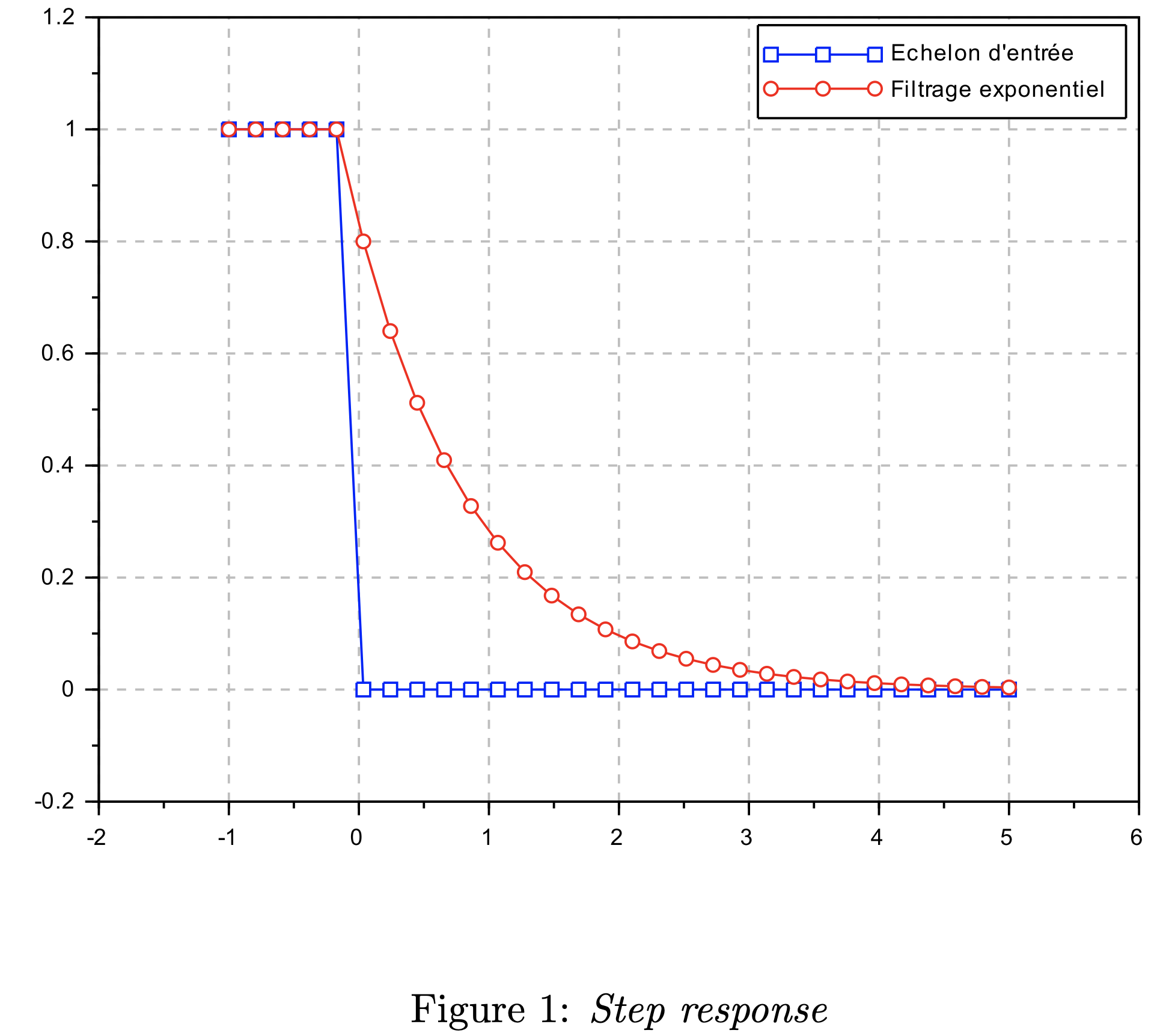
yn =(1−γ)yn−1 =(1−γ)ny0 =(1−γ)n supposing that y0 =1

2.Software Implementation:

If one uses a processor with floating point computing available, then the imple- mentation is trivial and correspond directly to the equation (1) :

y = (1 – alpha) * y + alpha * x;
where y is used both as an accumulator and as an output variable.

3. Deploying the algorithm on STM32:

We start of by creating a header file and name it First_Order_IIR_Filter.h

Inside this header file, we shall use a structure that holds the alpha and output values as following:

typedef struct
	{
	float alpha;
	float out;

	}FirstOrderIIR;

and two functions that shall initialize the filter and calculate the output as following:

void FirstOrderIIRFilter_Init(FirstOrderIIR *filter, float alpha);
float FirstOrderIRR_Calculate(FirstOrderIIR *filter, float in);

Hence, the header file is as following:

#ifndef FIRST_ORDER_IIR_FILTER_H_
#define FIRST_ORDER_IIR_FILTER_H_


typedef struct
	{
	float alpha;
	float out;

	}FirstOrderIIR;

void FirstOrderIIRFilter_Init(FirstOrderIIR *filter, float alpha);
float FirstOrderIRR_Calculate(FirstOrderIIR *filter, float in);

#endif /* FIRST_ORDER_IIR_FILTER_H_ */

Next, we create source file with same name of the header file.

For the initializing function, we shall first check if the alpha value is between 0 and 1 and set the output to zero

void FirstOrderIIRFilter_Init(FirstOrderIIR *filter, float alpha)
	{
	if(alpha<0.0f){alpha=0.0f;}
	else if (alpha>1.0f){alpha=1.0f;}
	else {filter->alpha=alpha;}
	filter->out=0.0f;
	}

For the calculation, we can use the equation from the software implementation as following:

float FirstOrderIRR_Calculate(FirstOrderIIR *filter, float in)
	{

	filter->out=(1.0f-filter->alpha)*in+(filter->alpha)*filter->out;


	return filter->out;
	}

For the output, HMC5883L Magnetic Field Sensor is used and you can get the code from here.

4. Code:

You can download the code from here: